Artificial Intelligence Neural Networks & Transformers
Neural Networks
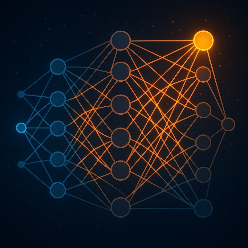
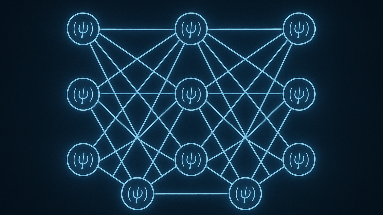
AI Neural Network showing pathways being triggered during calculations
An artificial neural network is a type of machine learning model inspired by the way biological brains process information. It’s built from layers of interconnected units called neurons, each performing simple mathematical operations, but collectively capable of learning very complex patterns.
1. Structure
A typical neural network has three main parts:
- Input Layer Receives raw data (numbers, images, text embeddings, etc.).Each neuron represents one feature or measurement from the input.
- Hidden Layers: One or more layers between input and output. Each neuron: Multiplies incoming signals by a weight. Adds a bias term. Passes the result through a non-linear activation function (e.g., ReLU, sigmoid, tanh). Hidden layers transform the input into increasingly abstract features.
- Output Layer Produces the network’s prediction. For classification: outputs probabilities for each class. For regression: outputs a continuous value.
2. How It Learns
The learning process is called training, and it happens in steps:
- Forward Pass Data flows from input → hidden layers → output. Predictions are compared to the correct answers using a loss function (e.g., cross-entropy, mean squared error).
- Backward Pass (Backpropagation) The network calculates how much each weight contributed to the error. Uses gradients to know the direction to adjust weights.
- Optimization An optimizer (e.g., SGD, Adam) updates the weights slightly to reduce the error. This process repeats many times (epochs) until the network learns the mapping from inputs to outputs.
3. Key Concepts
- Weights & Biases → The “memory” of the network.
- Activation Functions → Allow the network to model non-linear relationships.
- Overfitting → When the network memorizes training data instead of learning general patterns.
- Regularization → Techniques like dropout or weight decay to prevent overfitting.
4. Variations
- Feedforward Neural Networks (FNNs) → Data moves one way, no loops.
- Convolutional Neural Networks (CNNs) → Specialized for images and spatial data.
- Recurrent Neural Networks (RNNs) → Specialized for sequences (time series, language).
- Transformers → Advanced sequence models replacing many RNN uses.
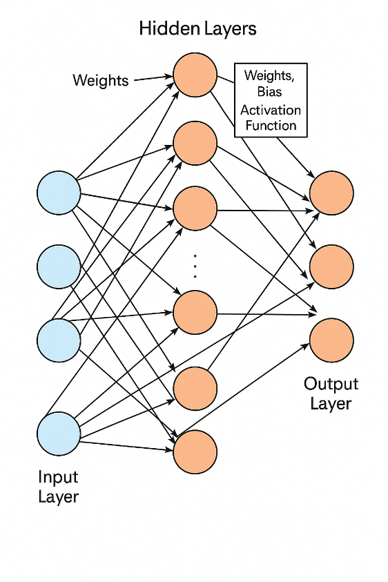
Illustration of a Neural Network with input blocks, hidden layers, and outputs
Loss Function
In artificial intelligence, specifically within neural networks, a loss function quantifies the discrepancy between the network’s predicted output and the actual, desired output (ground truth). It serves as a measure of how “wrong” the model’s predictions are. The primary goal during the training of a neural network is to minimize this loss function.
-
Prediction and Ground Truth:
The neural network processes input data and produces a prediction. This prediction is then compared to the known correct answer, also known as the ground truth or target label.
-
Calculating the Error:
The loss function takes both the predicted output and the ground truth as input and calculates a numerical value representing the “error” or “loss.” Different loss functions are used for different types of tasks. For example:
-
- Regression tasks: (predicting continuous values) often use Mean Squared Error (MSE) or Mean Absolute Error (MAE).
- Classification tasks: (predicting categories) commonly employ Cross-Entropy Loss (Binary Cross-Entropy for two classes, Categorical Cross-Entropy for multiple classes).
Training neural networks involves finding set of parameters θ that minimize a loss function
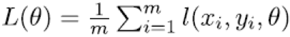
Function for determining the Loss function using Theta
Here, xi refers to the input, yi refers to the output data label, and m is the number of samples in the training batch. This minimization is typically performed using a variant of stochastic gradient descent. Let θ* denote the final parameter values after training. Since θ can have millions of parameters, we can’t visualize the loss function against all the dimensions of θ. To visualize a slice of this loss function, we pick two random directions ή and δ with the same dimension as θ and plot the function against α and β.
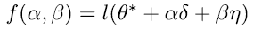
Function for visualizing a slice of the Loss function
Here α and β are scalars that vary across a suitable range on the x and y-axes. The density of the plot is determined by the sampling step size.
-
Guiding Optimization:
The calculated loss value provides a clear signal to the neural network about its performance. A higher loss indicates a greater discrepancy between prediction and reality, while a lower loss signifies better accuracy.
-
Backpropagation and Gradient Descent:
The loss value is then used in conjunction with backpropagation, an algorithm that calculates the gradients of the loss function with respect to each of the network’s parameters (weights and biases). These gradients indicate the direction and magnitude of change needed for each parameter to reduce the loss. An optimization algorithm, such as gradient descent, then uses these gradients to update the network’s parameters iteratively, aiming to minimize the loss function and improve the model’s predictive accuracy over time.
Transformer Network
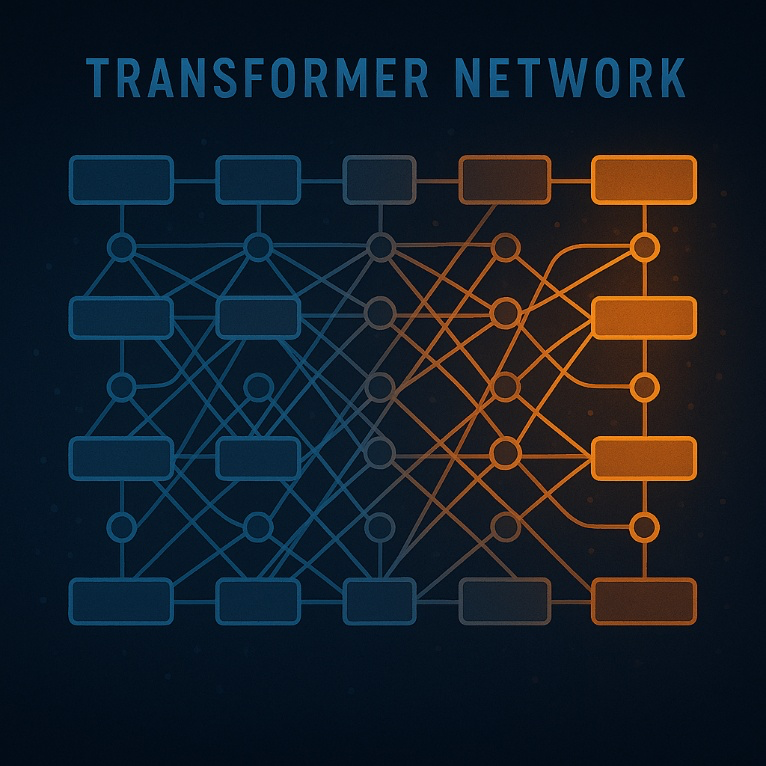
Transformer network showing pathways being triggered during calculations
Rectangular Blocks
- Role: Represent data processing layers or modules inside the transformer.
- In a typical transformer, the Leftmost blocks (blue) could represent input tokens/embeddings (the vectorized representation of words, images, or other data). Middle blocks are transformer layers — these contain multi-head attention and feed-forward sublayers. The rightmost blocks (orange) are outputs — the processed embeddings, ready for prediction or the next stage.
Circles
- Role: Represent connection nodes where multiple pathways converge or branch.
- In an actual transformer computation: They can be thought of as attention heads, residual connections, or aggregation points where data from multiple sources is combined. They also visually emphasize that in transformers, each element can connect to many others, not just the next sequential element.
In short:
- Blocks = processing stages (embeddings, transformer layers, outputs).
- Circles = junction points representing the complex web of attention and data flow between layers.
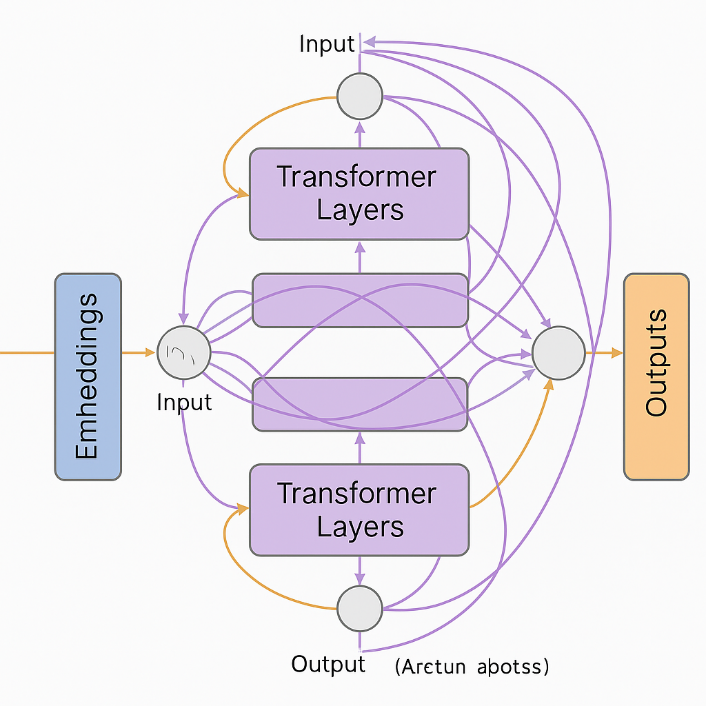
Illustration of a transformer with embedded blocks, attention layers, and outputs